| Graph
|
Directed graph (digraph)
|
Weighted graph
|
|---|
Graphs
Introduction
Some Notation
Graph 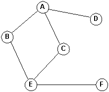
Directed graph (digraph) 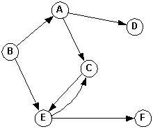
Weighted graph 
G = (V, E)
e = {v1, v2}
and v1 is the origin (source) and v2 is the terminus (destination).e = (v1, v2)
Strongly connected Weakly connected
Self-check:
Representing Graphs
Trees vs. Graphs
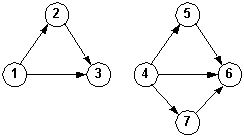
A B C
| Graph A | Graph B | Graph C | |||||||||||||||||||||||||||||||||||||||||||||||||||||||||||||||||||||||||||||||||||||||||||||||||||||||||||||||||||||||||||||||||||||||||||||||||||||
|---|---|---|---|---|---|---|---|---|---|---|---|---|---|---|---|---|---|---|---|---|---|---|---|---|---|---|---|---|---|---|---|---|---|---|---|---|---|---|---|---|---|---|---|---|---|---|---|---|---|---|---|---|---|---|---|---|---|---|---|---|---|---|---|---|---|---|---|---|---|---|---|---|---|---|---|---|---|---|---|---|---|---|---|---|---|---|---|---|---|---|---|---|---|---|---|---|---|---|---|---|---|---|---|---|---|---|---|---|---|---|---|---|---|---|---|---|---|---|---|---|---|---|---|---|---|---|---|---|---|---|---|---|---|---|---|---|---|---|---|---|---|---|---|---|---|---|---|---|---|---|---|
|
|
|
Note that for the weighted directed graph above we are using an integer matrix. (Could use other types
depending on the weights.)
| Unweighted digraph | Adjacency list | |
|---|---|---|
 |
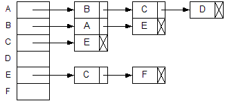 |
Self-check
Graph Traversals
Traversing a graph is a form of searching.
An algorithm for traversing a graph (assumes that vertices have a boolean visited field):
GraphSearch (G is the graph to search, v is the starting vertex)
  Put v into container C.
  While container C is not empty
    Remove a vertex, x, from container C
    If x has not been visited
      Visit x
      Set x.visited to TRUE
      For each vertex, w, adjacent to x
        If w has not been visited
          Put w into container C
        End If
      End For
    End If
  End While
End GraphSearch
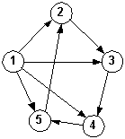
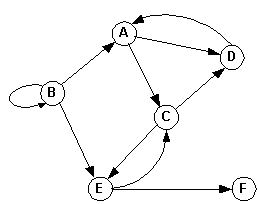
Given this graph, determine the sequence of nodes that are visited from different starting nodes.

Adjacency matrix: A B C D E F G H A 0 1 1 1 0 0 0 0 B 0 0 0 0 1 1 0 0 C 0 0 0 0 0 0 0 0 D 0 0 0 0 0 0 1 1 E 0 0 0 0 0 0 0 0 F 0 0 0 0 1 0 0 0 G 1 0 1 0 0 1 0 0 H 0 0 0 0 0 1 0 0
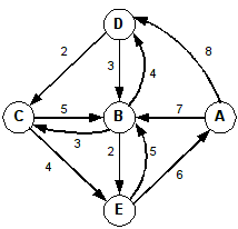
A weighted graph:
Example 3: Starting at A and sorting the adjacency set (maybe with a priority queue):
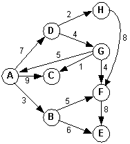
Adjacency matrix: A B C D E F G H A 0 3 9 7 0 0 0 0 B 0 0 0 0 6 5 0 0 C 0 0 0 0 0 0 0 0 D 0 0 0 0 0 0 4 2 E 0 0 0 0 0 0 0 0 F 0 0 0 0 8 0 0 0 G 5 0 1 0 0 4 0 0 H 0 0 0 0 0 8 0 0
Self-check What is the visited order starting at G using a queue? Using a stack? What is the visited order starting at H using a queue? Using a stack?
Notes:| Unoptimized | Optimized |
|---|---|
For each vertex, v, in graph, G GraphSearch (G, v) End For |
|
Self-check
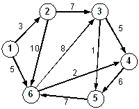
1. Given the graph below, what is the in-degree and out-degree of each node?
2. Starting at node A and using a depth-first search, in what order will the nodes be visited?
If a node has more than one neighbor, choose the edge with the larger value.
3. What is the order if you performed a breadth-first traversal instead?
4. What is the order if you choose the smaller edge for both depth-first and breadth-first traversals?
5. Is the graph strongly connected?
A Simple Implementation
The graph representation:
|
|
With actual bool values:
Graph G = { // Adjacency matrix                                       Adjacency list
            {false,  true,  true,  true, false, false, false, false},  // A-->B-->C-->D
            {false, false, false, false,  true,  true, false, false},  // B-->E-->F
            {false, false, false, false, false, false, false, false},  // C
            {false, false, false, false, false, false,  true,  true},  // D-->G-->H
            {false, false, false, false, false, false, false, false},  // E
            {false, false, false, false,  true, false, false, false},  // F-->E
            { true, false,  true, false, false,  true, false, false},  // G-->A-->C-->F
            {false, false, false, false, false,  true, false, false}   // H-->F
          };
void Visit(Vertex &v)
{
  cout << v.label << " ";
}

void GraphSearchStack1(Vertex *v, Vertex Vertices[])
{
  stack<Vertex *> C;

  C.push(v);                          // Put v into container C.
  while (!C.empty())                  // While (container C is not empty)
  {
    Vertex *x = C.top();              // Remove a vertex, x, from container C
    C.pop();
    if (!x->visited)                  // If (x has not been visited)
    {
      Visit(*x);                      // Visit x
      x->visited = true;              // Set x.visited to TRUE
      for (int i = 0; i < SIZE; i++)  // For each vertex, w,
      {
        if ((x->neighbors[i]) &&      //  (adjacent to x) and
            (!Vertices[i].visited))   //  (has not been visited)
          C.push(&Vertices[i]);       // Put w into container C
      }
    }
  }
}

void main()
{
  GraphSearchStack1(&Vertices[0], Vertices);
}
Using a queue instead of a stack: (slightly modified)for (int i = SIZE - 1; i >= 0; i--)
void GraphSearchQueue1(Graph G, Vertex *v, Vertex *vertices)
{
  int size = sizeof(G[0]);
  queue<Vertex *> C;        // uses a queue
  C.push(v);
  while (!C.empty())
  {
    Vertex *x = C.front();  // front() instead of top()
    C.pop();
    if (!x->visited)
    {
      Visit(*x);
      x->visited = true;
      for (int i = 0; i < size; i++)
      {
        if ((x->neighbors[i]) &&
            (!vertices[i].visited))
          C.push(&vertices[i]);
      }
    }
  }
}
Self-check
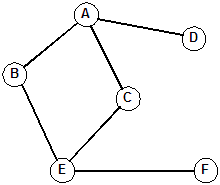
Given a connected, undirected graph G = (V, E), a tree that uses the edges, E, from G, and contains all of the vertices, V, is called a spanning tree for G.
There are two well-known algorithms for finding minimum spanning trees from a graph: Prim's algorithm and Kruskal's algorithm.
Examples:
| Original graph | Embedded tree | Tree |
|---|---|---|
|
|
|
|
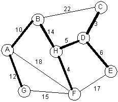
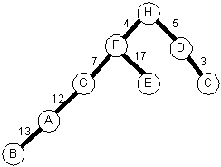
Prim's algorithm using a tree:
Starting at node A, the nodes will be added to the tree in this order:
A B G H F D C EStarting at node H, the nodes will be added to the tree in this order:
H F D C E B A GVideo review of Prim's algorithm.
The implementation is left as an exercise for the student.
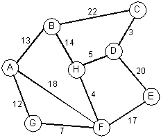
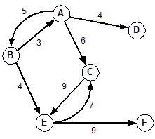
Kruskal's algorithm using a forest:
|
|
Priority queueEdge Weight ---- ------ C-D 3 H-F 4 H-D 5 D-E 6 A-B 10 A-G 12 B-H 14 G-F 15 F-E 17 A-F 18 B-C 22 |
The edges will be added in this order:
Changing a few weights: A-B(10 to 13), G-F(15 to 7) , D-E(6 to 20)C-D H-F H-D D-E A-B A-G B-H
| New graph | Priority queue | Graph with cycle | Embedded tree | |
|---|---|---|---|---|
|
Edge Weight ---- ------ C-D 3 H-F 4 H-D 5 G-F 7 A-G 12 A-B 13 B-H 14 F-E 17 A-F 18 D-E 20 B-C 22 |

|

|
The embedded tree:
Tree alone Another view Another view 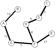

Video review of Kruskal's algorithm.
Elephant in the room: There is something that could make the implementation (as described above) of Kruskal's algorithm inefficient. (Union-Find algorithms).
The implementation is left as an exercise for the student.
More Spanning tree infoA Shortest Path Algorithm
Example graph and adjacency matrix:
| Graph | Adjacency matrix | Paths | ||||||||||||||||||||||||||||||||||||||||||||||||||
|---|---|---|---|---|---|---|---|---|---|---|---|---|---|---|---|---|---|---|---|---|---|---|---|---|---|---|---|---|---|---|---|---|---|---|---|---|---|---|---|---|---|---|---|---|---|---|---|---|---|---|---|---|
|
|
|
   Nodes      Cost
------------------
1 2 3 4 5      21
1 2 3 5        11
1 2 6 3 5      22
1 2 6 3 4 5    32
1 2 6 4 5      21
1 6 3 5        14
1 6 3 4 5      24
1 6 4 5        13
|
Given a source node, we can find the shortest distance to every other node in a graph.
Pseudocode for Dijkstra's algorithm:
Undirected Weighted Graph Paths and Costs From A 
Choose a node to be the source or starting point.
Initialize source to 0 cost and mark as evaluated.
Initialize all nodes to infinite cost from the source.

For each node, y, adjacent to source
  1. Relax the node. That is, set y's cost to the cost of all edges from source to y.
  2. Place y into a priority queue based on its total cost. (Lower is better)
  3. Add source node as predecessor of y.
End For

While there are nodes in the graph that haven't been evaluated
  Remove a node, x, from the PQ (lowest total cost)
  If the node has already been evaluated
    Discard the node
    Go to top of while
  Else
    Mark x as evaluated.
    For each neighbor, y, of x
      Relax y
      If new cost to reach y is less
        Update list of nodes (path) to y from source.
        Place y in the PQ.
      End If
    End For
  End If
End While
Video review of Dijkstra's algorithm.
Notes:


