Hashing
- Most of our algorithms deal with inserting, deleting, and finding
(searching/locating) items in a data structure (array, list, tree)
- The most fundamental operation is searching because most other operations depend on it
as well.
- Searching through arrays has complexities of O(N) and O(lg N). What
properties of the array cause these complexities?
- Locating an item by index is O(1)
- Searching through binary trees has complexities O(N) and O(lg N) as well. What
properties of the binary tree cause these complexities?
- Locating an item by index is O(lg N)
- Searching through a linked list has complexity O(N). (Singly- or doubly-linked)
- Locating an item by index is O(N)
- In the case of arrays and trees, the best we can do is O(lg N).
- Is this "As Good As It Gets" with data structures? Can we do better?
If we have to use a comparison function to identify an item (which could even be the built-in comparison operators),
the answer to "Can we do better?" is no. Binary search is the best we can do.
- What we need to be able to do is to find an item without having to compare it to other items.
- This is essentially how our searches (linear and binary) have been done thus far (comparing items).
- Given an item we'd like to:
- Perform some constant-time function, O(k)
- Locate the item in one step, O(1)
- Overall, this would give us a search complexity of O(k), which is Very Good.
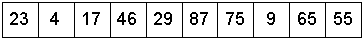
- Suppose we have an array of 10 integers.
- Assume that the values of any of the integers is in the range of 0 and 99.
- Two possible arrays could look like this:
Unsorted 10-element array (full):
Sorted 10-element array (full):

Complexity of searching? Pros/Cons?
A First Attempt
- Since we've stated that the values will be in the range 0..99, we
can simply create an array of that size (100) and store the items in the
array using their value as the index. (This is known as direct addressing.)
The value is called the key.
A 100-element array with 10 items (not full):
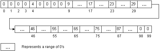
- We call this array a hash table. We call each element or cell a slot
(or bucket).
- Another name for a hash table is associative array, dictionary, or map.
- Storing/locating an item in this way is a key-based
algorithm. (Given a key, we can quickly find an item.)
- In this example, since all values are unique, we don't even need to store the value (it's implied by
its position).
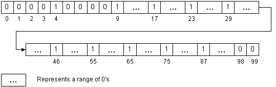
- We simply mark that slot with a 1, indicating the item's
presence.
- If the item is not present, we mark it with a 0. (Assume all slots
were initialized to 0 when we created the array.)
A 100-element array with 10 items (not full) marking with a 1 or 0:
What is the complexity of this approach? Pros/Cons? Limitations?
Suppose we want to store social security numbers?
- Note that if we wanted to have duplicates, we could simply use a count in the array instead of a 1 or 0. In other words,
if we stored the value 4 in the array 7 times, we would put the value 7 in slot 4:

Also, since these are just the keys, we could store the data outside (external) of the array and just store pointers
to the data along with the keys.
Given this Student structure:
struct Student
{
  string Name; // Maybe last and/or first
  long Year;   // 1 - 4
  float GPA;   // 0.00 - 4.00
  long ID;     // social security number, 000-00-0000 .. 999-99-9999
};
- To use the above techniques with this data, we need a way to
uniquely identify each Student.
- This means we need a key.
- Typically, we use all or part of the data itself as a key.
- If some portion of the data is unique, it is a good candidate for a key.
- If nothing about the data is unique, we may need to add information to the data to be used as a key.
- The Student struct has several potential key elements: (U is the Universal Set, the range of values)
- Name - Character array; uniqueness depends on size of student body (U can be quite large)
- Year - Small integer, unlikely to be unique (U is very small)
- GPA - Floating point, unlikely to be unique (U is small)
- ID - Relatively large integer, guaranteed to be unique (U is very large)
- Some combination of the above. (U can be customized)
The ID appears to be the best candidate:
- We could create an array that can contain all possible IDs (social security numbers).
- This array would have to have at least 999,999,999 elements!! (9-digits: XXX-XX-XXXX)
- Each 9-digit number would be an index into this (very) large array.
- Each element would be the size of a Student struct. (Probably at least 32 bytes)
- Clearly, this won't work well for at least two reasons:
- The size of the array would have to be at least 32 gigabytes.
- 99.9999% of the array will be empty.
Using a Portion of the ID
- We decide to use just a "few" of the digits.
- Which digits? (e.g first 3, first 4, last 4, middle 5)
- What are the limitations of these choices?
- Can we overcome these limitations?
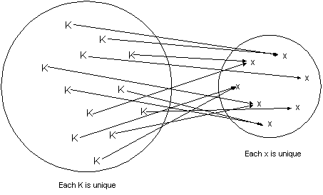
Hash functions are functions in the normal (mathematical) sense of the word (i.e. given some input, produce one output):
- Essentially, a hash function is an operation that maps one (large) set
of values into another, (usually smaller) set of values.
- Therefore, a hash function is a many-to-one mapping. (Two different inputs can have the same output.)
| Mapping a larger set into a smaller set: | Mapping into a hash table: |
|---|
|

|
- More specifically, this function maps a value (key of any type) into an
index (an integer) by performing arithmetic operations on the key.
-
The resulting hashed integer indexes into a (hash) table.
In this way, it is used as a way to lookup array elements quickly, O(1). (Arrays provide random access, aka
constant-time access)
In our Student example above, the key is the social security number
and the index is the result of applying the hash function. If H
is a hash function, and K is a key,
H(K) --> index
So, given a hash function SSHashFirst4, we can map social security
numbers into a set of indices. (SSHashFirst4 simply extracts and returns the first 4 digits):
SSHashFirst4(525334568) --> 5253  !!!
SSHashFirst4(559304056) --> 5593
SSHashFirst4(167782345) --> 1677
SSHashFirst4(525387000) --> 5253  !!!
SSHashFirst4(552559999) --> 5525
Or, given a hash function SSHashLast4, we can map social security
numbers into a different set of indices. (SSHashLast4 extracts the last 4 digits):
SSHashLast4(525334568) --> 4568
SSHashLast4(559304056) --> 4056
SSHashLast4(167782345) --> 2345
SSHashLast4(525387000) --> 7000
SSHashLast4(552559999) --> 9999
Graphically:
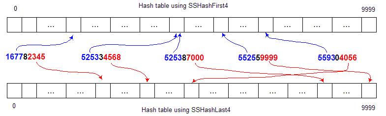
These trivial hash functions could be implemented like this:
unsigned SSHashFirst4(unsigned SSNumber)
{
  return SSNumber / 100000;  // return first 4 digits
}

unsigned SSHashLast4(unsigned SSNumber)
{
  return SSNumber % 10000;  // return last 4 digits
}
- There are at least two (related) potential problems with the SSHashFirst4 function. What are they?
- The SSHashLast4 function suffers from these problems, although to a lesser degree. Why?
- Positive side:
- We no longer need an array that must be large enough to hold the entire range of values.
- Our hash function is simple and fast. (In reality, hash functions are not quite this simple,
but they tend to be pretty fast.)
- When two or more keys hash to the same value, we call it a collision.
- It turns out that there are techniques to deal with collisions and the techniques are
collision resolution.
A note about hash functions: A good hash function will map keys uniformly and randomly into the
full range of indices. More on this later...
To be clear: The keys (input) used in a hash table must be unique. However, the resulting
hashed values (output) do not have to be unique (and often are not).
There are two parts to hash-based algorithms that implementations must deal with:
- Computing the hash function to produce an index from a key
- Dealing with the inevitable collisions
- One type of collision resolution policy is called linear probing.
- The basic idea is that if a slot is already occupied, we simply move to the next unoccupied slot.
- Looking for unoccupied slots is called probing. (Anytime you search for a slot using the hashed value, it's considered a probe.)
- This method of collision resolution is called open-addressing.
- Open addressing methods are used when the data itself is stored in the hash table (array).
As a simple example, we'll use single letters (A - Z) as keys for some larger data structure. Also, to keep things
simple, and to apply our hash function knowledge, we'll assume that our hash table has only 7 slots.
(Aside: What if the hash table had 26 slots?)
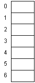
|
Each letter (key) will be its position in the alphabet (e.g. A1, B2, ..., Z26)
Our hash function will simply be something like this:
H(K) = K % 7 (the key modulo 7)
So A1 maps to 1, G7 maps to 0, H8 maps to 1, T20 maps to 6, etc.
Notice the significance of the value 7 (the table size). This property will be used in all of our hash functions.
|
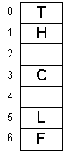
We want to insert the following keys into our hash table:
S19, P16, I9, N14, A1, L12
Our hash function will map the keys to indices like this:
H(S) = 5   (19 % 7)
H(P) = 2   (16 % 7)
H(I) = 2   ( 9 % 7)
H(N) = 0   (14 % 7)
H(A) = 1   ( 1 % 7)
H(L) = 5   (12 % 7)
- Using linear probing to resolve collisions, what would the hash table look like during and after
the insertions of the letters above?
- How many probes would be performed?
- What happens when we try to lookup (find) I9? How about B2?
- What if we inserted T20 into the table?
- What happens when we now try to lookup B2?
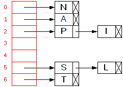
- Another example: Using linear probing to resolve collisions, what would the hash table look like during and after
the insertions of the letters:
F6, L12, E5, T20, C3, H8
Self-check: What does the hash table look like after inserting the 6 letters above?
How many probes were required?
The hash tables after inserting the letters above.
Notes:
- The direction of the linear probe is not important. (We could search forward or backward, but must be consistent.)
- We can't have duplicate keys, although two keys can map (hash) to the same index.
- All of the data is stored directly in the hash table (the array of slots).
- The number of items in the table (slots occupied), N, divided by the size of the table, M, is
the load factor
  Items in table (N)
  ------------------- = Load factor
   Size of table (M)
- If the table is sparsely populated, searching is fast since we'd expect to perform one
or two probes.
- If the table is nearly full, we will be spending most of our time resolving collisions. O(N) in worst case.
What is the worst case?
- Probing for an open slot handles collisions, but won't help if we run out of slots.
- Collisions tend to form groups of items called clusters.
- Clusters have a tendency to grow quickly. (Snowball effect.)
- Remember this:
The load factor determines the efficiency of the hash table.
Probability of forming/growing clusters:
- What are the chances of forming a cluster if there is one item in the table?
- What are the chances of forming a cluster if there are two items in the table?
- Three items? Four?
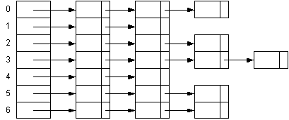
Clustering diagrams
Clusters affect probing (and should be avoided):
- The average number of probes to find an item (called a hit).
- The average number of probes to discover an item doesn't exist (called a miss).
- The load factor affects the performance significantly.
- Knuth derived formulas (non-trivially) that show how probing is directly related to the load factor, where
x is the load factor for a non-full table:
| Average number of probes for a hit: | | 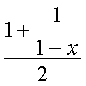 |
| |
| Average number of probes for a miss: | |  |
Plugging in values for the load factor, x, in the equations leads to this table:
           Load      Number of Probes
          Factor       Hit      Miss
-------------------------------------
  Nearly   .05        1.03      1.05
  empty    .10        1.06      1.12
           .15        1.09      1.19
           .20        1.13      1.28
           .25        1.17      1.39
           .30        1.21      1.52
           .35        1.27      1.68
           .40        1.33      1.89
           .45        1.41      2.15
  Half     .50        1.50      2.50
  full     .55        1.61      2.97
           .60        1.75      3.62
           .65        1.93      4.58
           .67        2.02      5.09
           .70        2.17      6.06
           .75        2.50      8.50
           .80        3.00     13.00
           .85        3.83     22.72
  Nearly   .90        5.50     50.50
  full     .95       10.50    200.50
Note:
As the load factor of the table approaches 1, the values tend to lose accuracy. However, in practice
you would never allow a hash table to get this full. So the values are accurate
enough when the table has a reasonable load factor.
The fundamental problem with linear probing is that all of the probes trace the same sequence (stride).
- Quadratic Probing: Probe 1, 4, 9, 16, 25, 36, etc. (Primary vs. Secondary clustering)
- Pseudo-random Probing: Probe by a random value. Must use key as the seed to ensure repeatability.
- Double Hashing: Use another (different) hash function to determine the probe sequence.
Hash function:  P(K) --> Primary hash gives starting point (index into the table)
Probe function: S(K) --> Secondary hash gives the stride (offset for subsequent probes)

P(K) is the Primary Hash and is calculated once for searches.
S(K) is the Secondary Hash and is calculated once only if there was a collision with P(K)

First probe is just the primary hash: P(K), 2nd Probe: P(K) + S(K), 3rd Probe: P(K) + 2S(K),
                                            4th Probe: P(K) + 3S(K) etc.
Double hashing performance: (formulas derived by Guibas and Szemeredi)
| Average number of probes for a hit: | |  |
| |
| Average number of probes for a miss: | |  |
                        Linear Probing       Double Hashing
             Load      Number of Probes     Number of Probes
            Factor%      Hit      Miss        Hit      Miss
------------------------------------------------------------
   Nearly      5        1.03      1.05       1.03      1.05
   empty      10        1.06      1.12       1.05      1.11
              15        1.09      1.19       1.08      1.18
              20        1.13      1.28       1.12      1.25
              25        1.17      1.39       1.15      1.33
              30        1.21      1.52       1.19      1.43
              35        1.27      1.68       1.23      1.54
              40        1.33      1.89       1.28      1.67
              45        1.41      2.15       1.33      1.82
   Half       50        1.50      2.50       1.39      2.00
   full       55        1.61      2.97       1.45      2.22
              60        1.75      3.62       1.53      2.50
              65        1.93      4.58       1.62      2.86
              70        2.17      6.06       1.72      3.33
              75        2.50      8.50       1.85      4.00
              80        3.00     13.00       2.01      5.00
              85        3.83     22.72       2.23      6.67
   Nearly     90        5.50     50.50       2.56     10.00
   full       95       10.50    200.50       3.15     20.00
Full table
Video review - Answers the question: Why is the tablesize a prime number?
- The performance of the hash table algorithms depend on the load factor of the table.
- Tables must not get full (or near full) or performance degrades.
- If we cannot determine the amount of data we expect (and hence the optimal size of the hash table),
we may need to grow it at runtime.
- This essentially means creating a new table and re-inserting all of the items.
- Expanding the table is costly, but is done infrequently.
- The cost is amortized over the run time of the algorithm.
- Much like how an ObjectAllocator works.
- Growing the table is similar to how a std::vector grows.
- Need to reinsert vs. simply copying old elements to new space.
- This is the difference between average case and worst case.
- ATM machine vs. Air-traffic control
Run-time issues:
- Performance profile can be erratic. (Similar to the ObjectAllocator or std::vector)
- Worst case is pretty bad, but rare and acceptable in many situations.
- Can also "shrink" the table if it becomes too sparse.
Video review - Inserting, growing, and deleting items.
Given the table containing the keys:
F6, L12, E5, T20, C3, H8
What happens to our search algorithm if we delete an item?
Question: How many clusters are in the diagram on the left?
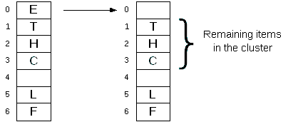
- After deleting E we search for key T (with hash value 6).
- Performing a linear probe from its hash value we arrive at an empty slot and conclude it isn't in the table.
- Deleting an item from a cluster presents a problem as the deleted item could be part of a
linear probing sequence.
Handling Deletions (Two Policies)
1. Marking slots as deleted: (MARK)
2. Adjusting the table: (PACK)
- Another solution is to "adjust" the table after a deletion.
- This is how an array or vector works.
(We don't mark an item deleted nor leave a "hole" in the array. We shift items.)
- For each item after the deleted item that's in the cluster:
- mark its slot as unoccupied
- Insert() it back into the table. (It will likely end up in a different slot.)
Results of re-inserting the cluster:
For relatively sparse tables the number of re-insertions is small. This is simply because the size of the clusters
are very small. (Maybe 2 or 3 elements.)
Self-check:What does the hash table look like after deleting the
letter F and re-inserting the cluster (PACK)?
Note: The performance of an open-addressed hash table is directly related
to the size of the clusters. The larger the clusters, the more comparisons that are required.
Smaller clusters require fewer comparisons.
Video review - Reinserting items after a deletion.
- With the open-addressing scheme, the data is stored in the hash table itself.
- In another scheme, called closed-addressing, the data is stored outside of the hash table.
- This method is also called chaining (or separate chaining)
- Instead of storing items in the hash table (in the slot indexed by the hashed key),
we store them on a linked list.
- The hash table simply contains pointers to the first item in each list.
The previous example would create a table with chains that look like this:
|
|
S19, P16, I9, N14, A1, L12
H(S) = 5   (19 % 7)
H(P) = 2   (16 % 7)
H(I) = 2   ( 9 % 7)
H(N) = 0   (14 % 7)
H(A) = 1   ( 1 % 7)
H(L) = 5   (12 % 7)
|
- The hash table now contains pointers (to nodes) instead of the data.
- Our data structure has been somewhat reduced to an array of singly-linked lists.
- Where do we insert into the list? Front/back/middle? Sorted? Will it matter? When?
- Splay (caching) hash tables???
Notes on Chaining:
- We never run out of space (technically, limited to available [virtual] memory)
- More allocations required for nodes. (Is that a problem?)
- Implementing insert and delete is trivial. (Compare to insert/delete on open-addressing hash table above.)
- Since we must ensure there are no duplicates, we must always look for an item before adding (inserting) it.
- Most time is spent searching through the linked lists.
- What is the worst case complexity for finding an item? Depends on the hash function.
- Complexity with a poor hash function? O(N), Why/When?
- Complexity with a good hash function? O(N/M), Depends on the load factor. (What is a good hash function?)
Complexity of Chaining
Recall the performance of linear probing:
- With linear probing we minimize probing by keeping the hash table around 2/3 full.
- This gave us an average of two probes (average cluster size of 3) for a successful search and five for an unsuccessful one.
- Note that these are constants, not related to the size of the data set. O(k)
With chaining:
There is no concept of "2/3 full".
Load factor is still calculated the same as before, but now it is likely to be greater than 1.
Think of the load factor as being the average length of the lists. (Given a good hash function, of course).
This example has a load factor of 2.86 (N/M, 20/7):
Complexity is the same as it was for singly-linked lists.
Why average complexity and not worst case here?
What looks better, linear probing or chaining? (Depends, pros and cons of both)
Self-check:
Given a table of size M that contains N items,
what is the average number of nodes visited in a successful search? Unsuccessful search?
Chaining demo GUI
- Until now, all of our keys have been numeric. (integers)
- Often, we don't have a numeric key (or the key is a composite)
- Many algorithms exist for hashing non-numeric keys (transforming non-numeric data to numeric data)
- Cyclic Redundancy Check
(CRC) algorithms can hash entire files. (CRC Calculator)
Run CRC on this data: 00110100111100101101110010100110
- Strings are widely used as keys (sometimes the key is the data or part of the data)
Note: The size of the table in the following examples is 211.
A simple (and naive) hash function for hashing strings:
unsigned SimpleHash(const char *Key, unsigned TableSize)
{
    // Initial value of hash
  unsigned hash = 0;

    // Process each char in the string
  while (*Key)
  {
      // Add in current char
    hash += *Key;

      // Next char
    Key++;
  }

    // Modulo so hash is within the table
  return hash % TableSize;
}
Sample run (string, hash):
bat, 100
cat, 101
dat, 102
pam, 107
amp, 107
map, 107
tab, 100
tac, 101
tad, 102
DigiPen, 39
digipen, 103
DIGIPEN, 90
- Simple, efficient, converts strings into integers.
- Doesn't produce a good distribution
A better algorithm is Program 14.1 in the Sedgewick book:
int RSHash(const char *Key, int TableSize)
{
  int hash = 0;         // Initial value of hash
  int multiplier = 127; // Prevent anomalies

    // Process each char in the string
  while (*Key)
  {
      // Adjust hash total
    hash = hash * multiplier;

      // Add in current char and mod result
    hash = (hash + *Key) % TableSize;

      // Next char
    Key++;
  }

    // Hash is within 0 - (TableSize - 1)
  return hash;
}
Sample run (string, hash):
bat, 27
cat, 120
dat, 2
pam, 56
amp, 188
map, 202
tab, 206
tac, 207
tad, 208
DigiPen, 162
digipen, 140
DIGIPEN, 198
- Produces a good distribution
- More complex, but not too bad
- Multiplier compensates for non-prime TableSize if table size is multiple/power of 2
A more complex hash function invented by P.J. Weinberger. It's a classic example.
int PJWHash(const char *Key, int TableSize)
{
    // Initial value of hash
  int hash = 0;

    // Process each char in the string
  while (*Key)
  {
      // Shift hash left 4
    hash = (hash << 4);

      // Add in current char
    hash = hash + (*Key);

      // Get the four high-order bits
    int bits = hash & 0xF0000000;

      // If any of the four bits are non-zero,
    if (bits)
    {
        // Shift the four bits right 24 positions (...bbbb0000)
        // and XOR them back in to the hash
      hash = hash ^ (bits >> 24);

        // Now, XOR the four bits back in (sets them all to 0)
      hash = hash ^ bits;
    }

      // Next char
    Key++;
  }

    // Modulo so hash is within the table
  return hash % TableSize;
}
Sample run (string, hash):
bat, 170
cat, 4
dat, 49
pam, 160
amp, 102
map, 28
tab, 118
tac, 119
tad, 120
DigiPen, 12
digipen, 154
DIGIPEN, 91
- Produces a good distribution
- More complex, but not too bad
A "pseudo-universal" hash function (Program 14.2 in the Sedgewick book):
int UHash(const char *Key, int TableSize)
{
  int hash = 0;       // Initial value of hash
  int rand1 = 31415; // "Random" 1
  int rand2 = 27183; // "Random" 2

    // Process each char in string
  while (*Key)
  {
      // Multiply hash by random
    hash = hash * rand1;

      // Add in current char, keep within TableSize
    hash = (hash + *Key) % TableSize;

      // Update rand1 for next "random" number
    rand1 = (rand1 * rand2) % (TableSize - 1);

      // Next char
    Key++;
  }

    // Account for possible negative values
  if (hash < 0)
    hash = hash + TableSize;

    // Hash value is within 0 - TableSize - 1
  return hash;
}
Sample run (string, hash):
bat, 163
cat, 162
dat, 161
pam, 142
amp, 67
map, 148
tab, 127
tac, 128
tad, 129
DigiPen, 142
digipen, 64
DIGIPEN, 96
Comparisons (Tablesize is 211)
| SimpleHash |
| RSHash |
| PJWHash |
| UHash |
bat, 100
cat, 101
dat, 102
pam, 107
amp, 107
map, 107
tab, 100
tac, 101
tad, 102
DigiPen, 39
digipen, 103
DIGIPEN, 90
|
|
bat, 27
cat, 120
dat, 2
pam, 56
amp, 188
map, 202
tab, 206
tac, 207
tad, 208
DigiPen, 162
digipen, 140
DIGIPEN, 198
|
|
bat, 170
cat, 4
dat, 49
pam, 160
amp, 102
map, 28
tab, 118
tac, 119
tad, 120
DigiPen, 12
digipen, 154
DIGIPEN, 91
|
|
bat, 163
cat, 162
dat, 161
pam, 142
amp, 67
map, 148
tab, 127
tac, 128
tad, 129
DigiPen, 142
digipen, 64
DIGIPEN, 96
|
Other data:
Hash function performance and distribution
Things to consider:
- The data size is known (min, max)
- Don't have to grow the table, just size it to get the desired load factor.
- Much like using reserve with a std::vector
- The operations are known (insert, remove, search)
- e.g. there are no (or very few) deletions; don't have to worry about re-inserting (PACK) the cluster
- Performance matters more than memory (time/space trade-off)
- Linear probing vs. double-hashing
- Open-addressing vs. closed-addressing (chaining)
Probing with open-addressing:
- If the table is sparse (and memory is available), linear probing (stride is 1) is very fast, however:
- Performance can degrade rapidly once clusters start forming.
- One cluster can affect another cluster.
- Performance
- Double hashing uses memory more efficiently (smaller table, denser), costs a little more
to compute secondary hash (stride).
- For sparse tables, linear probing and double hashing require about the same number of probes, but
double hashing will take more time since it must compute a second hash.
- For nearly full tables, double hashing is better than linear probing, due to the less
likelihood of collisions (secondary clustering).
- For efficiency, tables using linear probing should remain less that 2/3 full.
- If the size of the data is large, this requires a lot of extra unused storage.
- Algorithms for inserting/deleting are peculiar. (i.e. There are no "off-the-shelf"
containers/functions to implement the algorithm.)
- Using linear probing with the table (array) may be more cache-friendly than double-hashing.
- Open-addressing makes serialization easier (no pointers to store).
Chaining with closed-addressing:
- Has the potential benefit that removing an item is trivial.
- No re-inserting clusters or marking the slot as deleted.
- Trivial to implement (vector and linked list algorithms/containers readily available).
- Node allocation can be expensive, but can be implemented efficiently with a memory manager (ObjectAllocator).
- Extra storage required for the table (data is stored outside the table)
- Extra storage required for "next" pointers in the lists.
- The amount of extra storage required is constant so if the size of the data
is large, the overhead is not (unlike with open-addressing)
- Only allocate memory for actual data (no reserved space like open-addressing).
- Degrades gracefully as the average length of each lists grows. (No snowballing effect, i.e. clustering)
- Each chain is independent of the others.
- Even with a poor hash function the performance won't be as bad as open-addressing
(where clusters are not independent of each other).
- Lists could be sorted using a BST or other data structure.
- However, not very useful in practice due to the short length of the lists.
- Although, the HashMap class in Java uses a balanced BST.
- Using a vector (dynamic array) instead of a linked list has some benefits (e.g. cache-friendly).
- Linked lists are not very cache-friendly.
- Serialization is problematic (pointers).
Final thoughts:
- Hash tables rely on the fact that the data is uniformly and randomly distributed.
- Since we cannot control the data that is provided (from the user), we must ensure
that it is randomly distributed by hashing it.
- Open-addressed hash tables whose size is a prime number help to ensure good distribution when double-hashing.
- Table sizes that are a power of 2 also work well if the stride is an odd number.
- Since the data is not sorted in any meaningful way, operations such as displaying
all items in a sorted fashion are expensive.
- Use another data structure for that operation (e.g. red-black tree).
- Hash-like algorithms are used in other areas as well.
- E.g. Cryptography and pseudo-random number generators
- Hash tables are widely used in computer science for things like databases, caches, and
string pools.
Interesting links:
This idea of randomization leads to randomized algorithms
(used in skip lists) or Monte Carlo
algorithms such as Buffon's Needles
Buffon.exe from efg's Computer Lab