Heaps
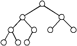
- A heap is a complete binary tree where each child's value (key) is less than (or equal) to
it's parent value (key).
- Recall that a complete tree is a balanced tree and that all nodes on the bottom level are stored
as far left as possible:
| Complete Binary Tree | | Heap |
|---|
|
|
|
|
|
|
|
 | |  |
- Any node's value in the tree is larger than or equal to all of its children's values.
- A tree is said to be heap-ordered if it has these properties.
- We'll see that a heap can be implemented in structures other than binary trees.
- Technically, you could heap-order any tree, but the implementations will result in
significant improvements if we require a complete tree.
The heap property
- The benefit of a heap is that the largest value is always at the root.
- Locating this value can be done in O(1) (constant) time.
- Like stacks and queues, has push and pop.
- We typically want to remove the largest value (the root).
- We must replace the root with another node, but which one?
- The choice of the replacement node dictates the complexity of the implementation.
- Choose a node that has little or no effect on the structure of the tree.
- This will be the last node in the tree, which will preserve the completeness of the tree.
- Replacing the root will likely cause the heap property to be lost, so we must heapify the
tree. (Much like balancing other trees after an insertion or deletion.)
Note that a heap is not simply a "sorted" tree or linked list. The largest value is first (root), but
the rest of the tree may (and usually will) not be completely ordered and may contain duplicates.
(Children are less than or equal to their parent.)
This is a desirable property when we're only interested in the largest value. Much easier to simply
locate the largest item rather than to sort the entire structure. This is the idea behind priority queues.
Priority Queue example using arrays and linked lists.
The complexity of the priority queue is directly related to the data structure used to represent it.
Some algorithms that make use of priority queues are Dijkstra's algorithm, Kruskal's algorithm, and the
A* (A-Star) algorithm.
Example:
This tree is a heap because it has the properties described above:

Removing the largest element
- Easy to do because it's at the root.
- This leaves a vacancy at the root that must be filled.

- Fill this vacancy with the last node in the tree.
- It is safe to remove the last node because it will never have any children. (It's a leaf, afterall)
- It also preserves the completeness of the tree.
- If the tree no longer has the heap property, we need to restore that property.

To heapify the tree after removing the root and replacing it, simply swap the root
with the larger of its children:

Continue this process until the swapping no longer results in a child node being larger than
its parent:

- The tree now has the heap property again.
- What is the cost of heapifying the tree? (i.e. How many swaps in the worst case?)
- By definition, heaps (complete trees) are guaranteed to be balanced.
- Note that removing the last element (right-most node on bottom level) doesn't
destroy the complete-ness of the tree.
Removing the largest element again
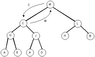
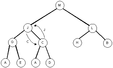
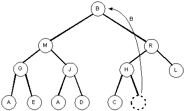
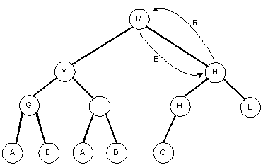
After removing the root node R from the previous tree, we have to heapify the tree.
| Step 1: | Step 2: |
|---|

|

|
| Step 3: | Step 4: |
|---|

|

|
Inserting into a heap
Inserting F into the tree causes no problems. The tree maintains the heap property. Inserting
into the right-most position on the bottom level preserves the completeness as well.

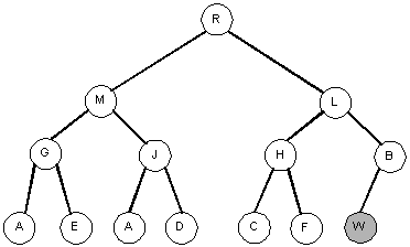
Inserting W into the tree causes the heap property to be lost: (W > B)

Heapifying the tree is similar to how it was done before except that we will work from
the bottom up (instead of the top down).
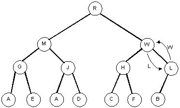
W is larger than B, so we swap the nodes:

W is larger than L, so we swap the nodes:

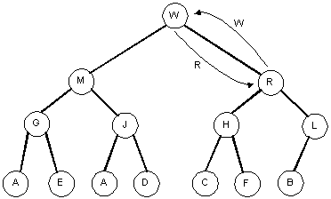
W is larger than R, so we swap the nodes.

- We are now at the root so we are done and the heap property has been restored.
- Since we traverse the tree in both directions (top-bottom, bottom-top), we might
want to use a parent pointer (back pointer) for efficiency (depending on the implementation).
- The worst-case time for heapifying after insertion is the same as removal.
Self-check: Draw the tree after removing W from the last tree above.
Then, draw the tree after inserting A, N, and P into the tree.
- Elephant in the room: How do we find the last element in the tree?
- Numbering the nodes in the tree using a level-order traversal:
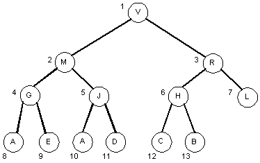
- What do you notice about the children and their numbers?
- Growth-rate comparison
- Complete binary trees have a very nice property that they can be easily represented by compact arrays.
- These arrays are time- and space-efficient.
- This means that finding the last node in the tree/array takes O(k) time.
- This is even better than O(lg N) time.
- Also, there is no wasted space in the array. (The arrays are packed, not sparse).
Example:
Again, if we number the nodes by position in the complete binary tree using level-order (breadth-first) traversal we arrive at these
values:

- Think of these positions as being an "index" into the tree.
- The root is at index 1, the left child of the root is at index 2, the right child of the root is at index 3, etc.
- The key as to why this is efficient is in recognizing the relationship between a parent and its
children.
- This leads to the following discoveries:
Given the "index", i, of a node,
- the node's left child is at index 2i
- the node's right child is at index 2i + 1
- the node's parent is at index i / 2 (using integer division)
- the node is a leaf if 2i > N, where N is the number of nodes in the tree.
- This allows us to find all of this information in constant time.
- For example, node J at index 5:
- The left child is at index 2i (10).
- The right child is at index 2i + 1 (11).
- The parent is at index i / 2 (2, integer division).
- The node is not a leaf because 2i (10) is less than 13.
Given this parent-child relationship, we can simply represent the complete binary tree above as an array.

We will leave the first slot empty to make the arithmetic easier.
The root of the tree is V and its left and right children are M and R, respectively:

Node J has left and right children A and D, respectively:

|

|
Node L is a leaf and has no children: 2i > N (i = 7 and N = 13)

Removing the root
Original heap:
Remove largest element:
Move last node to root:
R is larger than M, so swap B and R:
L is larger than H, so swap B and L:
B is a leaf, (2 * 7 > 12), so we're done.
Inserting into the heap
Insert F, heap property is preserved (F < H)
Insert W, heap property is violated (W > B)
Swap W and B, heap property is still violated:
Swap W and L, heap property is still violated:
Swap W and R. W is at the root, so we are done.
Notes:
- Using a sorted array requires O(N) copies (shifts) to maintain the sort.
- Using a heap requires O(lgN) copies (swaps) to maintain the heap.
- This is a huge difference.
- When N is 1,000, that's 1,000 vs. 10.
- When N is 1,000,000 that's 1,000,000 vs. 20.
- When N is 1,000,000,000 that's 1,000,000,000 vs. 30.
Self check Implementing a heap using an array is left as an exercise for the student.
Using the STL to create a heap from an array:
| std::make_heap | std::priority_queue |
|---|
void f1()
{
  srand(10);
  std::vector<int> v;
  for (int i = 0; i < 20; i++)
    v.push_back(RandomInt(10, 99));

  std::cout << "vector: ";
  PrintArray(&v[0], v.size());

  std::cout << "  heap: ";
  std::make_heap(v.begin(), v.end());
  PrintArray(&v[0], v.size());

  std::cout << "\npop, print, heapify\n";
  while (!v.empty())
  {
      // print "top", pop, re-heapify
    std::cout << v[0] << "  ";

      // Expensive operation: O(N) due to shifting
    v.erase(v.begin());

    std::make_heap(v.begin(), v.end());
  }
}
|
void f2()
{
  srand(10);
  std::vector<int> v;
  for (int i = 0; i < 20; i++)
    v.push_back(RandomInt(10, 99));

  std::cout << "Using a priority queue:\n";
  std::priority_queue<int> pq(v.begin(), v.end());
  while (!pq.empty())
  {
    std::cout << pq.top() << "  ";

      // Cheap operation: O(lg N), no shifting
    pq.pop();
  }
}
|
Output:
vector: 81  79  42  24  27  36  72  52  36  19  64  21  13  24  43  92  51  79  74  40
  heap: 92  81  72  79  64  36  43  52  79  40  27  21  13  24  42  24  51  36  74  19

pop, print, re-heapify...
92  81  79  79  74  72  64  52  51  43  42  40  36  36  27  24  24  21  19  13

Using a priority queue:
92  81  79  79  74  72  64  52  51  43  42  40  36  36  27  24  24  21  19  13
With 40,000 elements:
f1() runs in about 5.2 seconds
f2() runs in about 0.007 seconds

with 50,000,000 items, f2() runs in about 5.2 seconds.
An example showing how to use operator> with a priority queue:
| std::priority_queue (with operator>) | |
|---|
void f2b()
{
  srand(10);
  std::vector<int> v;
  for (int i = 0; i < 20; i++)
    v.push_back(RandomInt(10, 99));

  std::cout << "Using PQ with operator> instead of operator<:";

    // Use operator> instead of operator<  (orders the elements from small to large)
  std::greater<int> comparor;

    // Construct PQ with desired sort order
  std::priority_queue<int, std::vector<int>, std::greater<int>> pq(v.begin(), v.end(), comparor);
  while (!pq.empty())
  {
    std::cout << pq.top() << "  ";
    pq.pop();
  }
}
|
|
Output:
Using PQ with operator> instead of operator<:
11  15  27  27  28  41  45  48  58  58  68  70  73  81  84  87  93  93  95  98
Final thoughts:
- Implementing heaps using arrays may be more cache-friendly than trees.
- Although, copying data could be expensive.
- Less memory is required because no pointers are needed (the indexes are implicit).
- Don't need to dynamically allocate each node.
- Heaps form the logic behind
Heapsort, (Go figure), which has worst-case O(N lg N)
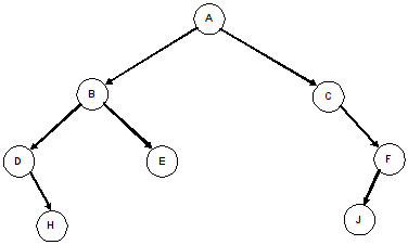
Self check: Fill in the array from the tree below such that it will allow
efficient (constant-time) access to a node's children and parent. Yes, there will
be "holes" in the array for the missing nodes.
Note: This isn't a heap, just a mapping of tree nodes into array slots.
Tree:

Array:


